Sometimes a customer specification requires you demonstrate your equipment can withstand shock or vibration loading. This could involve physical testing, engineering analysis, or both. If this is not a common requirement or if you generally subcontract out this type of work, you may be unfamiliar with the different types of finite element analyses (FEA) used to qualify equipment for shock and vibration. This article discusses the various types of finite element analyses used to evaluate equipment for shock and vibration loading, how they differ from each other, and when they are typically used.

There are a number of different types of finite element analysis methods used in evaluating equipment and structures for shock and vibration loads. These include: time-history (transient), static-g, modal, harmonic, response spectrum, and random vibration.

Time-History (Transient) Analyses

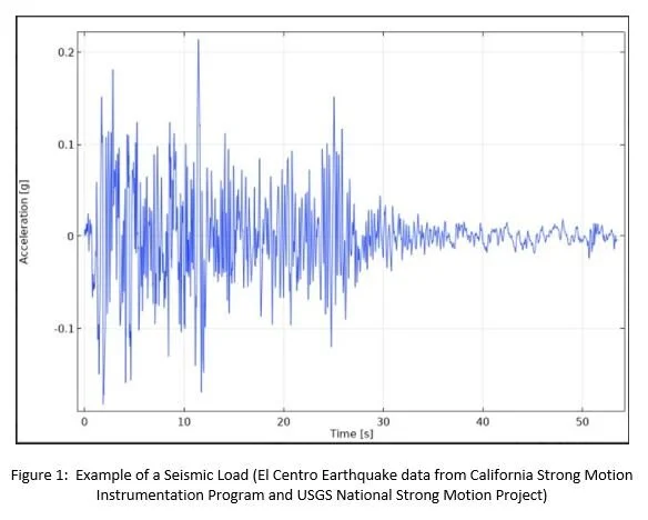
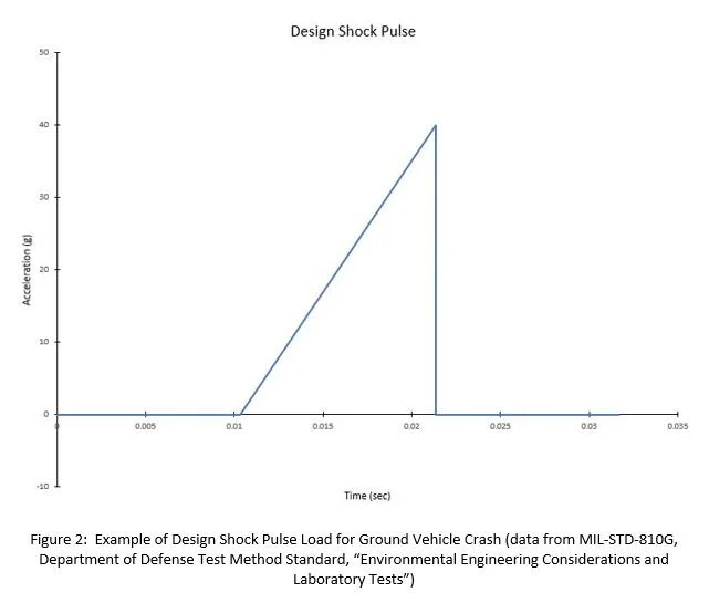
Time-history analyses, also referred to as transient analyses, consist of applying a time-varying load on a finite element model of a structure or equipment, and determining how it responds over some length of time. Figures 1 and 2 show examples of shock and vibration loading for use in a time-history analysis. Figure 1 is data from an actual seismic event. Figure 2 is the input for a design impact load.

Time-history analyses can generally produce results that are a good representation of how the equipment or structure will actually respond to an applied load. As such, one would think that a time-history analysis would be the preferred type of finite element analysis method in evaluating shock and vibration loading, and would be common.

This however, is not always the case. Performing a time-history analysis using FEA requires results to be calculated at a sufficient number of distinct points in time to accurately define the input load and predict the equipment or structure’s response to the load. It is not unusual for time-history analyses to have results at increments of 0.00001 seconds.

As a result, time-history analyses often mean long computer run times, large results files using up computer space, and significant engineering man-hours poring through the results. Whether or not performing a time-history analysis is considered reasonable usually depends on the size of the finite element model (i.e., number of nodes and elements) and duration of the applied load. Larger finite element models will have longer run times and use more computer space. The longer the applied load, the more time steps requiring distinct results. As such, time-history analyses of equipment subjected to impact loads lasting milliseconds such as shown in Figure 2 are common, while time-history analyses of equipment subjected to a seismic load lasting nearly a minute such as shown in Figure 1 are a rarity.

Static-g Analyses

A static-g analysis consists of applying a constant acceleration (in g’s or other units) to a finite element model and determining its response.

Since the applied load in this type of analysis is constant, the results are the maximum response of the structure or equipment for the applied load. Technically, this method of evaluation is not a dynamic analysis method. Rather it is a static analysis method using a constant load that is approximating a time-varying load. The magnitude of the static (constant) acceleration is usually based on a typical expected load or a “worst-case” scenario.

From a computer resource and engineering effort standpoint, static-g analyses are the quickest and simplest type of shock and vibration analysis method. Because of this, static-g analyses are common. Static-g analyses are also sometimes used to get “ball park” results to “zero in” on a design prior to running a more complicated shock and vibration analysis. Static-g analyses are typically used for equipment and structures that respond to shock and vibration loads as a rigid body.

Static-g analyses are commonly used in evaluating transportation loads, impact loads, and seismic loads.

Modal Analyses

A modal analysis is used to determine the natural frequencies of a structure. A modal analysis in of itself will not determine how a structure or equipment will respond to shock or vibration loads. Rather it is typically used to make sure the natural frequencies of a structure will not be excited by a cyclic load, such as ensuring resonance will not occur in a platform supporting rotating equipment. A modal analysis is required prior to running harmonic, response spectrum, and random vibration analyses.

Harmonic Analyses

Harmonic analyses are often used to evaluate equipment subjected to sinusoidally varying loads. This could be to evaluate for a load occurring at a specific frequency or to evaluate the equipment for a load over a range of frequencies. An example of a graph of a harmonic load is shown in Figure 3. A modal analysis of the equipment is required prior to conducting a harmonic analysis.

Harmonic analyses are common in evaluating rotating equipment such as motors and fans.

Response Spectrum Analyses

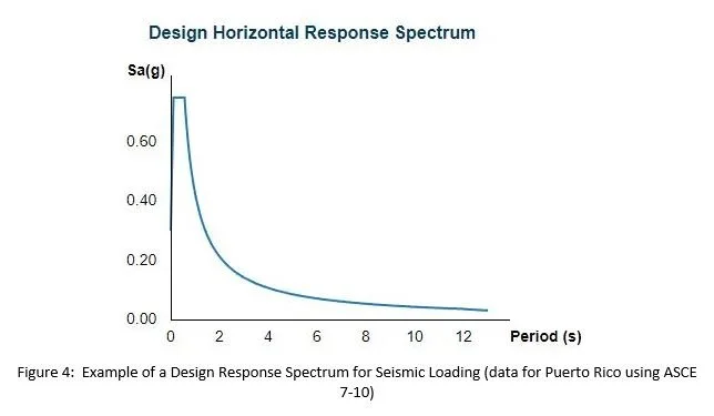
As discussed above, the applied load in a time-history (transient) analysis varies with time and can often use significant computer and engineering resources. Since the load and results vary with time it occurs in what is referred to as the time domain. A response spectrum analysis is a simplified analysis method that uses a time-varying load that has been converted into the frequency domain. In a response spectrum analysis, the applied load varies with frequency (or period), as opposed to time, as shown in Figure 4.

With a response spectrum analysis, a modal analysis is first performed to determine the natural frequencies of the equipment or structure. The response of the equipment or structure at the various natural frequencies identified by the modal analysis are scaled by the magnitude of the input load at that particular frequency and how much of the equipment’s mass is active at that particular frequency (i.e., the participation factor). All of these individual responses at the various natural frequencies are then combined, usually using the square root sum of the squares (SRSS) method. The net result is the maximum response of the structure or equipment for the applied load.

Response spectrum analyses are typically used where a static-g analysis is not appropriate, such as when a structure is not considered rigid, or when the duration of the load is not short (e.g., occurs over seconds, not milliseconds). Response spectrum analyses are fairly common in evaluating structures and equipment for seismic loading.

Random Vibration Analyses

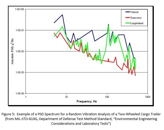
A random vibration analysis is used to determine how a structure or equipment will respond to loads whose magnitude and frequency of occurring are random. Random vibration analyses are similar to response spectrum analyses in that the load is defined in the frequency domain. However, the spectrum for a random vibration analysis (referred to as a power spectral density, or PSD) is provided in units of the applied load squared per Hertz (e.g., g2/Hz), versus frequency. An example of a spectrum for a random vibration analysis is shown in Figure 5.

The spectrum used in random vibration analyses represent the probability of a particular load of a certain magnitude occurring at a particular frequency. As such, random vibration analyses are non-deterministic, or probabilistic.

Like a response spectrum analysis, a modal analysis is first performed to determine the natural frequencies of the equipment or structure. While the math behind random vibration analyses is quite involved, random vibration analyses are similar to spectrum analyses in that the response of the equipment or structure is a function of the response at various natural frequencies, the input spectrum (PSD), and how much of the equipment’s mass is active at that particular frequency (i.e., the participation factor). All of these individual responses at the various natural frequencies are then combined, usually using the square root sum of the squares (SRSS) method. However, since a random vibration analysis is probabilistic, the net result for the maximum response of the structure or equipment for the applied load will be different depending on whether you are viewing 1-sigma, 2-sigma, or 3-sigma results.

Random vibration analyses are typically used in evaluating equipment for loads that are random in nature, such as transportation loads.

Closing Remarks

The characteristics of the applied load (e.g., harmonic, random, short-duration, etc.) will typically determine which analysis method of shock and vibration is appropriate, if not already specified by the customer.

Harmonic, response spectrum, and random vibration analyses all require a prior modal analysis. While time-history and static-g analyses do not require a modal analysis, performing a modal analysis is always a good idea to gain insight on how the structure will respond. The appropriateness of a static-g analysis is often based on the equipment or structure responding as a rigid body within a particular frequency range. A modal analysis will confirm this.

While short-duration shock and vibration loads are often evaluated using a time-history (transient) analysis, longer duration loads are typically evaluated using either a static-g analysis or a response spectrum analysis.

Lastly, the amount of time spent modeling and defining the applied loads generally doesn’t differ much between the different analysis methods. The greatest differences in engineering effort occur in evaluating the results, with static-g analyses taking the least amount of time and time-history analyses taking the most.

Blog

Evaluating for Shock and Vibration Using FEA